Above 80 km

Height, first

Conventional layer boundaries, not sharp walls. The tropopause is near 8 km in the polar winter and near 18 km in the tropics; 12 km is a midlatitude figure. The ozone layer is not its own shell. It is a concentration of ozone inside the stratosphere, mostly about 15–35 km, with the peak often near 25 km. Below 40 km this drawing is stretched so the mountains, the aircraft, and that ozone band can be seen. From 40 km up, the spacing is even. The pictures mark altitude. They are not drawn to size.

0

10

20

30

40

60

80

100

120

Ozone layerMesosphereLower thermosphereMeteorsCO₂ profiles

80 km · Mesosphere

Read one height in three units

80 km · 80,000 m · 49.7 mi

Mesosphere

Altitude

SurfaceMount EverestAirliner cruiseTropopause, midlatitudesOzone layerScientific balloonStratopauseCO₂ profiles bendMesopauseMeteors usually glowKármán lineTop of these profiles

Altitude of the same levels in kilometres, metres, and statute miles

Level	km	m	miles
Surface	0	0	0.0
Mount Everest	8.8	8,800	5.5
Airliner cruise	11	11,000	6.8
Tropopause, midlatitudes	12	12,000	7.5
Ozone layer	15–35	15,000–35,000	9.3–21.7
Scientific balloon	35	35,000	21.7
Stratopause	50	50,000	31.1
CO₂ profiles bend	80	80,000	49.7
Mesopause	85	85,000	52.8
Meteors usually glow	80–110	80,000–110,000	49.7–68.4
Kármán line	100	100,000	62.1
Top of these profiles	120	120,000	74.6

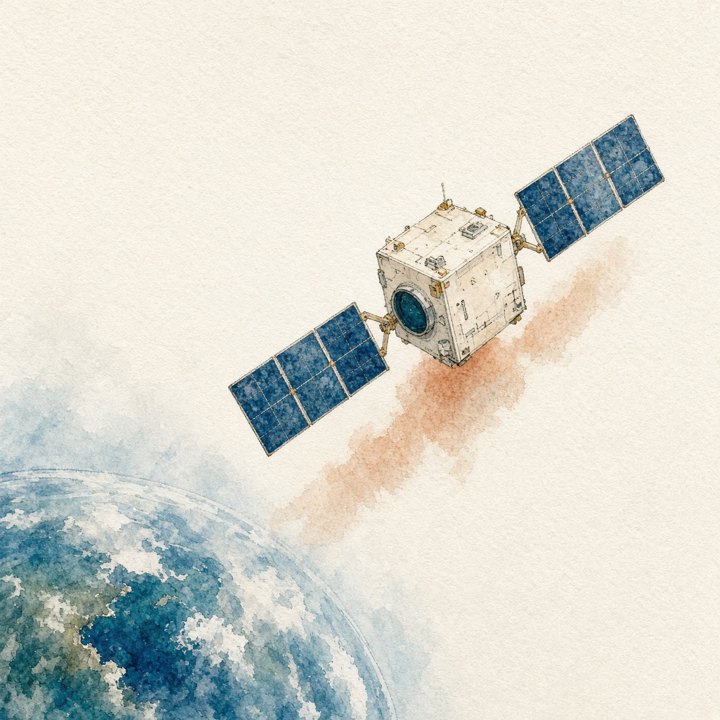
Above this chart. The International Space Station orbits near 400 km: 400,000 m, about 249 miles. That is more than three times the top of the profiles on this page. The satellite is drawn off the scale on purpose. Putting it at 120 km would be the wrong height.

The CO₂, water, and chlorine profiles sit between 60 and 120 km, marked by the teal edge of the column. Nothing in those profiles was collected by an aircraft.

What the figures actually show

The ink is traced from the printed figures and sampled every 2 km. It is not the Level-2 archive. ACE-FTS is a measurement. Every CMAM scenario is a model. Where lines overlap near 370 ppmv, a scenario that could not be separated by color is omitted. Scenario E (CO+OH slowed by 5) is one of those.

Molecule bench

A global-mean diffusion–chemistry column from 50 to 130 km. It is not CMAM and not WACCM. Eddy mixing, molecular diffusion, photolysis, and a few reactions are solved to steady state. The knee reported here is where the mixing ratio drops below 90% of its value at 65 km. Pressure is hydrostatic. The lower boundary is fixed.

Kzz chosen so CO₂ stays near 370 ppm through ~80 km and is down by ~10% near 90 km.

CO₂ leaves 90% of its 65 km value at 89 km. Argon, which is only inert and heavy, does it at 97 km. Water’s inert twin rises; real water is chemically gone much lower.

Findings

Ordered as an audit, not as a score. “Holds up” means the paper’s claim survives the check. Garcia et al. (2014, doi:10.1002/2013JD021208) is the intervening analysis that both of these results have to sit next to.

1. 01MethodBeagley 2010

   CO₂ was put in the same budget as water, methane and N₂O

   The discussion says H₂O, N₂O, CH₄ and CO₂ are all set by vertical transport balanced against chemical loss. That sentence is right for water, methane and nitrous oxide. It is the wrong budget for CO₂. The global-mean CO₂ profile is molecular diffusive separation against eddy mixing; photolysis is a minor term and changes CO₂ by less than about 10% above 100 km (Garcia et al., 2014). An inert gas with the mass of CO₂ falls off. An inert gas with the mass of water rises. Real water falls anyway, because Lyman-α destroys it.

2. 02ContradictionBeagley 2010

   The 13-day Lyman-α lifetime does not match the cross section in the same paper

   They adopt σ(CO₂) = 7.7×10⁻²⁰ cm² at Lyman-α, inside the 6.5–8.2×10⁻²⁰ cm² range they cite. A line-integrated solar flux of about 4×10¹¹ photons cm⁻² s⁻¹ then gives J ≈ 3×10⁻⁸ s⁻¹, a lifetime of roughly a year. Two pages later the dust argument uses 1/J ≈ 13 days at 80 km. Those two numbers differ by a factor of about 30. Night and zenith angle make the diurnal-mean lifetime longer, not shorter, so they do not close the gap. The claim that γ = 0.1 on meteoric smoke is 3–5 times faster than photolysis is ratioed to the 13-day figure. The calculator below uses their cross section and lets the flux vary.

3. 03MethodBeagley 2010

   Eddy diffusion was tested only at full strength and at zero

   Scenario A includes Hines Kzz. Scenario C sets it to zero. Nothing in between was run. Because molecular diffusion grows roughly exponentially with height, a factor of four in Kzz moves the CO₂ knee by about one scale height, ~10 km — the size of the discrepancy they are trying to explain. Scenario C did lower CO₂, and they say so. They then drop transport because zero was not a complete fit, and conclude a missing chemical sink. López-Puertas et al. (2000), which they cite, had already shown in one dimension that a modest Kzz (tens of m² s⁻¹) sets this profile.

4. 04MethodBeagley 2010

   Photolysis ×5 fits April at 30°N and is too strong in August

   Scenario B is their best CO₂ match at 30°N in April. The same factor is described as excessive in August: the model CO₂ then falls off too fast. CO in scenario B is high by a factor of about four to five, which is why they reject pure photolysis. A constant dust efficiency would not be mild in April and excessive in August. The residual changes with season, which is what transport does.

5. 05MethodBeagley 2010

   CO was allowed a larger error than the CO₂ knee they treated as decisive

   The control CO simulation is called adequate. In the same text it is ~30% low near 0.001 hPa in April and about a factor of two low there in August. The CO₂ offset of ~10 km is treated as requiring new physics. Garcia et al. (2014) read the same pair of symptoms the other way: too much constituent diffusion keeps CO₂ high and mixes CO down, and an O₂ cross section near 105–121 nm that is ~10× too large under-produces CO. Raising that photolysis by a factor of two to three fixes CO and barely moves CO₂, because photolysis is not the term that sets the knee.

6. 06MethodBeagley 2010

   γ = 0.1 is an assumption, and it would remove total carbon

   The dust estimate uses meteoric surface areas from Megner et al. (2008) and a mechanism pointed at Plane (2004). That literature is about metal atoms and ions on smoke, not a measured irreversible sink of CO₂. They set the reactive uptake coefficient to 0.1 so the lifetime becomes 9/γ hours and beats their 13-day photolysis. Photolysis converts CO₂ into CO, so CO + CO₂ stays put. A sink that sequesters carbon does not. The bench shows the difference. They never plotted the sum.

7. 07ContradictionBeagley 2010

   SABER v1.06 was preliminary, and the later retrieval changed the sign of the bias

   The paper says the SABER v1.06 CO₂ is not validated. In their Fig. 2 it lies about 20 ppmv above ACE above the knee, with the knee near 80 km. Rezac et al. (2015) validate the v2.0 two-channel retrieval: SABER is systematically lower than ACE, the mean difference is under 5% from 65 km to about 100 km, and it grows to about 20% at 110 km. The version change is as large as the offset used in 2010, and it points the other way. v1.06 cannot be cited as independent confirmation of the ACE knee.

8. 08ContradictionBeagley 2010

   The abstract’s CRISTA knee (~70 km) is stronger than the authors’ own caveat

   The abstract says the ACE knee near 78 km is higher than CRISTA-1 (~70 km), lower than SABER v1.06 (~80 km), and much lower than rockets. In the body they report that Kaufmann judged the CRISTA mixing ratio to depart significantly from its lower-atmosphere value only above 80 km. Rockets, as they plot them, put the knee near 87 km. The spread among observations is comparable to the 10 km model offset the abstract treats as a clear miss.

9. 09MethodBeagley 2010

   The ACE prior can slide the knee; the quoted percentage errors do not say otherwise

   CO₂ above ~60 km is forced toward a 5th-order polynomial, zero at the anchor where the mixing ratio is declared constant. That prior is exactly able to move the altitude of the bend. They estimate total error under 10% below 100 km, and about 16% systematic at 118.5 km, so the mixing ratio itself is not noise. A percentage error bar is not an error bar on the knee altitude. Two related weaknesses they do state: the instrument line shape is an empirical function “not based on any physical process,” and a 5 K temperature uncertainty above the mesopause “might be an underestimate.” The retrieval’s real strength is also stated correctly: only ground-state lines are used, so non-LTE is a smaller problem than for the emission sounders.

10. 10LimitBeagley 2010

    A good temperature field does not certify constituent Kzz

    Fig. 10 shows CMAM and ACE temperatures in reasonable agreement, and they infer that the resolved circulation is adequate. Constituent eddy diffusion is not fixed by that test. The Prandtl number in a gravity-wave scheme sets tracer diffusion relative to momentum and heat. Garcia et al. change it from 4 to 2, double Kzz, and lift thermospheric CO₂ into agreement without touching the chemistry. CMAM can have a credible temperature and still the wrong tracer diffusivity. ACE occultation sampling, which they discuss, adds a separate high-latitude bias.

11. 11LimitBeagley 2010

    A mis-plotted panel was caught in review

    In the ACPD discussion López-Puertas flagged Fig. 8a. The authors replied that the original panel had been mis-plotted. The published ACP figure is the correction. This is not evidence the final figure is still wrong. It is evidence these cross-sections were easy to get wrong, so a traced reproduction should not be treated as the Level-2 archive.

12. 12Holds upRezac 2015

    SABER versus ACE is inside the stated errors, and the bias is still systematic

    The comparison uses coincidences within ±5° latitude, ±10° longitude and ±4 hours (943 pairs on the symposium figure of this study). SABER’s two-channel CO₂ is daytime only; ACE is sunrise and sunset. From 65 to ~100 km the mean SABER−ACE difference is under 5%, growing to ~20% at 110 km, and SABER is the lower one. The same team’s accuracy table gives single-profile CO₂ uncertainties of 15, 15, 12, 21 and 32% at 70, 80, 90, 100 and 110 km. A 20% mean difference at 110 km fits inside 32%. The agreement claim holds. The low bias is real; it is just not larger than the error budget they published.

13. 13ContradictionRezac 2015

    “Within 5%” ends at 90 km in the key points and at ~100 km in the conclusions

    The key points say the mean SABER and ACE mixing ratios agree within 5% below 90 km, and up to 20% at 110 km. Section 5 says the mean difference is smaller than 5% from 65 to ~100 km, then 20% at 110 km. Both can be loosely true if the difference is a few percent through 100 km, but they are not the same sentence. The traced global means cross: SABER is slightly higher than ACE near 90 km (~337 vs ~323 ppmv) and lower at 110 km (~107 vs ~155 ppmv).

14. 14MethodRezac 2015

    SD-WACCM’s knee is ~5 km low, which is the opposite miss from CMAM

    The 10 November 2015 talk of this validation says the global-mean SABER and ACE profiles leave well-mixed values about 5 km higher than SD-WACCM, and asks whether eddy diffusion is too weak. It points at Garcia et al. (2014): reducing the Prandtl number from 4 to 2 increases Kzz and improves CO₂. The paper treats Prandtl number 4 as the standard WACCM setting and a tunable parameter, and the abstract leads with seasonal agreement. The bias is in the opposite direction from Beagley’s CMAM, whose knee was ~10 km too high. Two models missing on opposite sides of the observations is what an uncertain Kzz does. It is not evidence for a missing CO₂ sink.

15. 15Holds upRezac 2015

    They flagged an unphysical 400 ppmv ACE value near 30°N

    In the January zonal mean, ACE reaches 400 ppmv near 30°N. The paper calls it an outlier: the troposphere had not reached 400 ppm during 2004–2012. That is the correct call. The difference plot should not be read hard at that latitude.

16. 16MethodBoth

    Weight, temperature and chemistry move different gases in different directions

    Diffusive equilibrium changes a mixing ratio as exp[−(mᵢ − m_air)gz/(kT)]. CO₂ (44 u) and argon (40 u) fall. Helium (4 u) rises. Water (18 u) and methane (16 u) would rise if they were inert; both are destroyed by photolysis and oxidation well below the CO₂ knee, water sharply once Lyman-α is optically thin near 85–90 km, methane already through the lower mesosphere. HCl (36.5 u) is heavy, so total chlorine eventually separates, but HCl itself is also converted to atomic chlorine. CO (28 u) has almost no mass contrast with air; it increases because it is the product of CO₂ photolysis, not because it is light. Colder air strengthens the mass term (1/T) and shrinks the scale height. Pressure is not an independent knob: number density, which sets the molecular diffusion coefficient (D ∝ 1/n), follows from hydrostatic balance given T and the mean mass. Mean mass itself falls above ~100 km as atomic oxygen grows, so every contrast with air changes.